Kernel Density Estimation with Polars

André included in Data Science Dataframes Polars

2025-03-12 1137 words 6 minutes

Contents

Abstract

We will see how to use polars’ out of the box optimizations to make parallelized kernel density estimations. To this end, I created the polars_kde package, which is a polars plugin backed by some Rust code.

Note

At the time of writing the polars_kde package has version 0.1.4 and is available on pypi.

Info

By now, the standard reference for writing polars plugins is Marco Gorelli’s excellent tutorial here. If you want to learn how the internals of polars plugins work, please have a look at his tutorial.

Tip

Some advertisement: If you haven’t already checked out my other polars plugin polars_sim, make sure to have a look. The plugin enables very fast approximate joins on string columns (fuzzy matching but with a twist). The implementation is entirely written from scratch in Rust and uses n-gram vectorization of strings with a fast cosine similarity computation using sparse matrices.

Introduction

Kernel Density Estimation (KDE) is a non-parametric way to estimate the probability density function of a random variable. I recently created a basic marimo notebook on how to visualize feature distributions and drift over time, possibly grouped by another categorical variable, e.g. the target of a classifier. See my repository marimo_notebooks for more details or check out the interactive notebook here.

While working on this notebook, I realized that the computations usually involve multiple kde’s for different slices of the data. In order to have a polars built-in method to compute kde’s, I created the polars_kde package. This enables optimized computations and polars-native code (as opposed to for example using scipy).

The updated notebook with the new polars plugin in place can be found here.

If you (trust me) and want to run the notebook in your local environment, simply fire

        
uv tool run marimo edit https://github.com/schemaitat/marimo_notebooks/blob/main/notebook/feature_drift_fast.py

Note

The interactive marimo notebook uses the scipy implementation. The polars_kde package is not yet available as wasm build.

Interactive Marimo Notebook

Adding interactive marimo notebooks to a static blog.

Adding interactive marimo notebooks to a static blog is as easy as adding an iframe for wasm html files. See the docs. The marimo notebooks are self-contained and can be hosted on any static file server.

I integrated this into my workflow by adding a marimo folder containing all the notebooks. Then, each notebook is exported to a same named folder in the public folder (where the rendered blog html lives).

In my Jenkins pipeline, I install the notebooks as follows:

        
        
        
    
#!/bin/bash

if [ -z "$1" ]; then
    echo "Usage: $0 <output_dir>"
    echo "  output_dir: directory to store the rendered notebooks"
    exit 1
fi

output_dir=${1:-public}/marimo

# create a temp directory to store the rendered notebooks
mytmpdir=$(mktemp -d 2>/dev/null || mktemp -d -t 'mytmpdir')


if [ -d $output_dir ]; then
    echo "Output directory already exists. Clearing it."
    rm -rf $output_dir
else
    mkdir -p $output_dir
fi

for notebook in "marimo/*.py"; do
    # remove .py ending
    dir_name=$(basename $notebook)
    dir_name="${dir_name%.*}"
    echo -ne 'Y' | uv run marimo export html-wasm --sandbox --mode run $notebook -o $mytmpdir/$dir_name
    mv $mytmpdir/$dir_name ${output_dir}/$dir_name
done


trap "rm -rf $mytmpdir" EXIT SIGINT SIGTERM SIGQUIT SIGKILL

Rust side

On the rust side of things, all we need to do is wrapping an already existing functionality into a polars expression. Often, this is the standard approach on how to create polars plugins. Another example is for example the polars-reverse-geocode plugin.

        
        
        
    
use kernel_density_estimation::prelude::*;
use polars::prelude::*;
use polars_core::utils::align_chunks_binary;
use pyo3_polars::derive::polars_expr;
use serde::Deserialize;

#[derive(Deserialize)]
struct KdeKwargs {
    eval_points: Vec<f32>,
}

fn compute_kde(sample_points: Vec<f32>, eval_points: Vec<f32>) -> Vec<f32> {
    let kde = KernelDensityEstimator::new(sample_points, Silverman, Normal);
    kde.pdf(&eval_points)
}


#[polars_expr(output_type_func=same_output_type)]
fn kde_agg(inputs: &[Series], kwargs: KdeKwargs) -> PolarsResult<Series> {
    let values = &inputs[0].f32()?;
    let eval_points = kwargs.eval_points;

    let sample_points = values.into_no_null_iter().collect::<Vec<_>>();

    let samples = compute_kde(sample_points, eval_points);

    Ok(Series::new(PlSmallStr::EMPTY, samples))
}

Note

You see that I use Normal as kernel and Silverman as bandwidth estimator. This is a common default choice, but a future improvement would be to make these parameters configurable.

Examples

To get the basic idea, we start with a simple example. We have a dataframe with two columns, id and values. We group by id and compute the kde for the values column. We work with a fixed set of evaluation points, which are the points at which the kde is evaluated.

        
        
        
    
import polars as pl
import polars_kde as pk

eval_points = [0.1, 0.2, 0.3, 0.4, 0.5, 0.6, 0.7, 0.8, 0.9]

df = pl.DataFrame({
    "id" : [0,0,0,0, 1, 1],
    "values" : [0.1, 0.2, 0.3, 0.4, 0.5, 0.6]
},
schema = {
    "id" : pl.UInt32,
    "values" : pl.Float32
})

df_kde = df.group_by("id").agg(kde = pk.kde("values", eval_points = eval_points))
print(df_kde)

shape: (2, 2)
┌─────┬─────────────────────────────────┐
│ id  ┆ kde                             │
│ --- ┆ ---                             │
│ u32 ┆ list[f32]                       │
╞═════╪═════════════════════════════════╡
│ 1   ┆ [1.7249e-11, 0.000002, … 0.000… │
│ 0   ┆ [1.816287, 2.407217, … 1.1300e… │
└─────┴─────────────────────────────────┘

Now lets generate some more data and add a visualization:

        
        
        
    
import numpy as np
import polars as pl
import polars_kde as pk
import seaborn as sns

df = pl.DataFrame({
    "id" : np.random.randint(0, 10, 10_000),
    "values" : np.random.normal(0, 1, 10_000),
}).with_columns(
    values = pl.col("values") + pl.col("id") * 0.1
).cast({
    "values": pl.Float32
})

eval_points = [x/100 for x in range(-400, 400)]

df_kde = (
   df
  .group_by("id")
  .agg(
    kde = pk.kde("values", eval_points = eval_points),
  )
  .with_columns(
      # add the evaluation points as a column
      # for plotting
      eval_points=pl.lit(eval_points)
  )
  .explode("kde", "eval_points")
)

sns.lineplot(
    df_kde,
    x="eval_points",
    y="kde",
    hue="id",
)

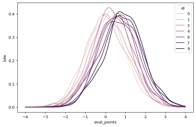
See also the Readme of the polars_kde for some more examples on varying evaluation points.

Note

The kde function works also on group_by_dynamic groups and is particularly useful for timeseries aggregations.

Speed

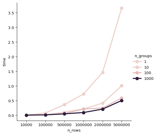
Especially, for large dataframes and many groups, the speedup is significant. Compared to the scipy implementation, the polars_kde is faster even for a single operation faster. For illustration, let us look at some boilerplate code that can be used to generate more benchmarks.

        
        
        
    
import numpy as np
import polars as pl
import polars_kde as pk
import seaborn as sns
import time

def benchmark(n_groups, n_rows):
    df = pl.DataFrame({
        "id" : np.random.randint(0, n_groups, n_rows),
        "values" : np.random.normal(0, 1, n_rows),
    }).with_columns(
        values = pl.col("values") + pl.col("id") * 0.1
    ).cast({
        "values": pl.Float32
    })

    eval_points = [x/100 for x in range(-50, 50)]

    start = time.time()
    df_kde = (
       df
      .group_by("id")
      .agg(
        kde = pk.kde("values", eval_points = eval_points),
      )
    )
    end = time.time()

    df_bench = pl.DataFrame({
      "n_groups": [n_groups],
      "n_rows": [n_rows],
      "time": [end - start]
    })

    return df_bench

bench_n_groups = [1, 10, 100, 1000]
bench_n_rows = [10_000, 100_000, 500_000, 1_000_000, 2_000_000, 5_000_000]

# Include this to generate the plot.
# Here, I added the output on my local machine with 8 cores,
# since the build agent is single core and we would not see
# any parallelization.

# df_bench = pl.concat([
#     benchmark(n_groups, n_rows)
#     for n_groups in bench_n_groups
#     for n_rows in bench_n_rows
# ])


# sns.catplot(
#     df_bench,
#     x="n_rows",
#     y="time",
#     hue="n_groups",
#     kind="point"
# )

Contents

Kernel Density Estimation with Polars

Introduction

Rust side

Examples

Speed

Benchmark on 8 cores.